Workflow Vignette#
This page shows what a complete panache run looks like from config file to
output, and demonstrates how plume detection varies across seasons and
threshold methods. All images were produced from real L4 SPM satellite data
(EUR-L4-SPIM-ATL-v01-fv01-OI) for 1 January 2024 (winter) and
1 July 2024 (summer). Each zone is shown under both the dynamic
gradient-based threshold and the global 95th-percentile (p95) threshold,
so the sensitivity difference between the two methods is immediately visible.
1. Prepare a config file#
Create a JSON config that points panache at your data. The simplest approach
is to use one of the four built-in zone presets:
{
  "zone": "GULF_OF_LION",
  "input_path": "/data/SEXTANT/SPM/",
  "bathymetry_path": "/data/bathymetry/Bathy_data.pkl",
  "output_dir": "/data/panache-output/GULF_OF_LION",
  "coast_shapefile": "/data/boundaries/gadm41_FRA_0.shp",
  "overwrite": false,
  "gif": true,
  "nb_cores": 4,
  "dynamic_threshold": false,
  "global_threshold_quantile": 0.95,
  "variable_name": "analysed_spim"
}
Key choices:
Key |
What to set |
|---|---|
|
One of |
|
Path to a folder of |
|
Path to the bathymetry pickle; downloaded automatically if absent |
|
|
|
Compute this percentile from the full scene and use it as the flood-fill threshold |
|
|
|
zlib compression level (1-9) applied to |
2. Run the pipeline#
panache gulf_of_lion_config.json
panache prints a progress line per file and reports the path to Results.csv
when the run completes.
3. Examine the outputs#
GULF_OF_LION/
├── Results.csv       ← batch statistics, one row per (day, river) + one 'ALL' zone-total row per day
├── PlumeMasks.nc      ← per-river + 'ALL' plume masks, one (river, lat, lon) slice per day
├── manifest.csv      ← status of every input file
├── GIF.gif           ← animated overview (when gif: true)
└── MAPS/
    └── 20240101-EUR-L4-SPIM-ATL-v01-fv01-OI.png
For a zone with N rivers (e.g. Gulf of Lion has 2: Grand Rhône and Petit
Rhône), each day contributes N+1 rows to Results.csv: one per river plus a
river='ALL' row carrying the combined-mask (union) statistics. Since a
river’s flood fill is entirely independent of its neighbours, two rivers’
masks can legitimately overlap; the n_pixel_shared_with_other_rivers column
makes that overlap auditable rather than silently double-counted if the
per-river rows are summed. Each row also carries a single SPM_threshold
value (that row’s own river; NaN on the ALL row) rather than one
SPM_threshold_<river> column per river as in versions before v0.5.0. See
Using PlumeMasks.nc to Extract Daily SPM Values for the matching PlumeMasks.nc layout.
As of v0.5.2, Results.csv also carries sum_SPM_in_the_plume_area (the raw
pixel-wise sum of SPM concentration, g m-3, over the finite-valued
plume pixels) alongside the existing mean_SPM_in_the_plume_area and
sd_SPM_in_the_plume_area. The mass column is now named
mass_SPM_in_the_plume_area_in_t (previously
mass_SPM_in_the_plume_area_in_g_m, which despite its name held kilograms)
and reports tonnes directly: sum_SPM_in_the_plume_area multiplied by the
per-pixel area and an assumed 1 m water-column depth. Cloud-gap pixels within
the mask are excluded from the sum and are not imputed, so they contribute
zero to the mass total.
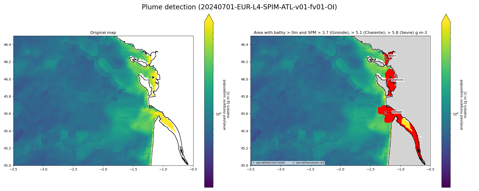
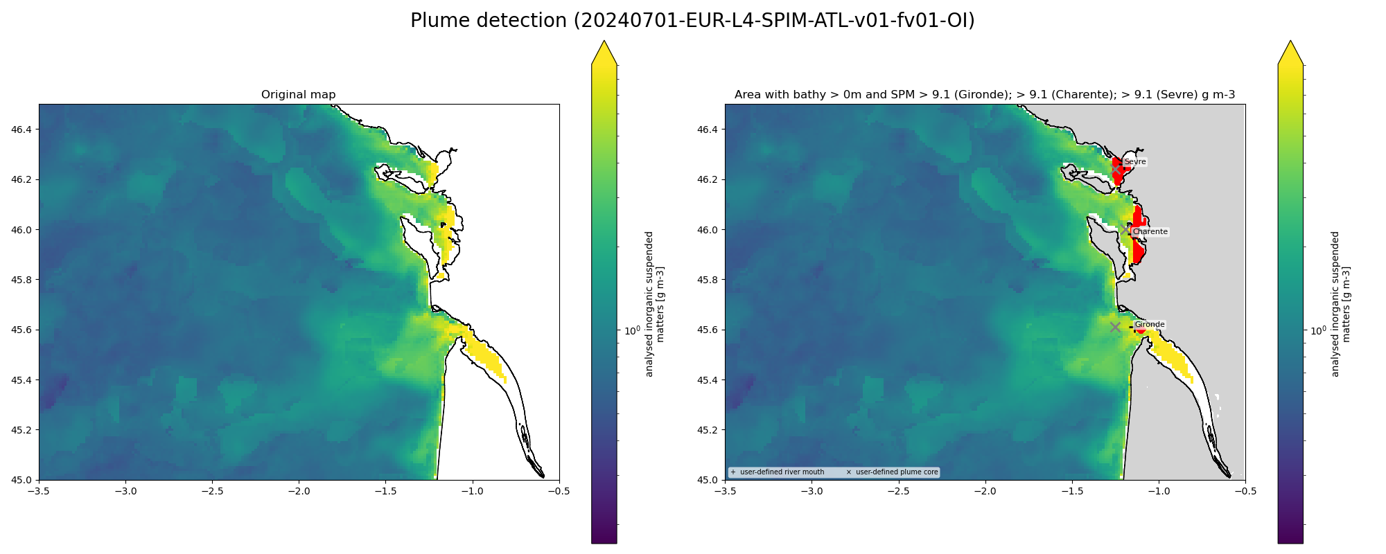
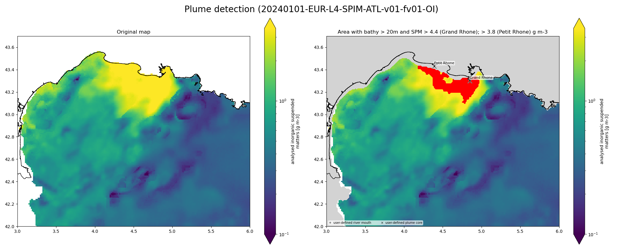
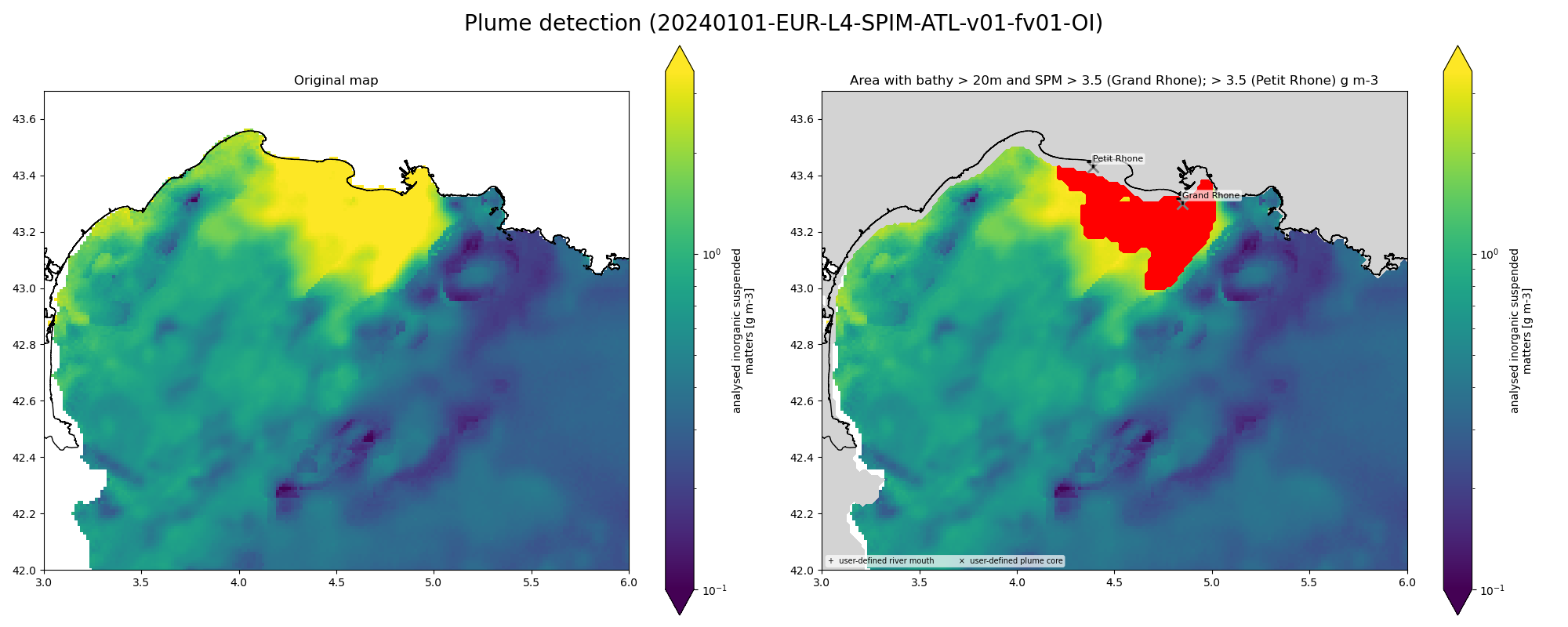
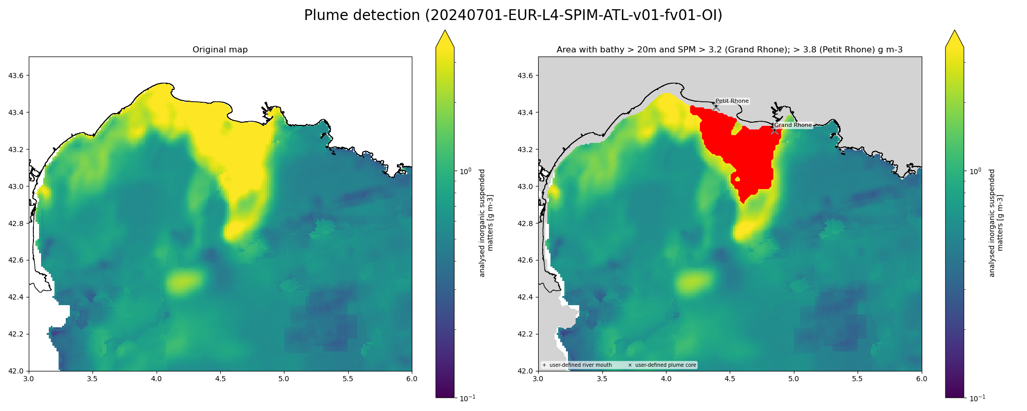
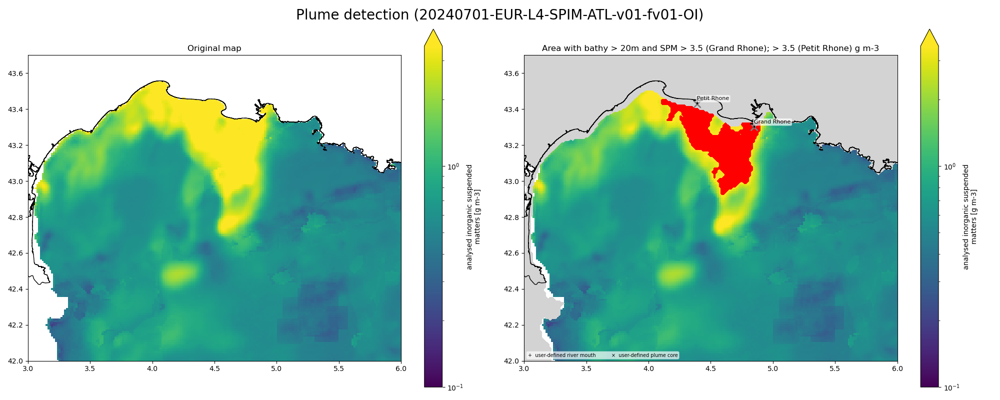
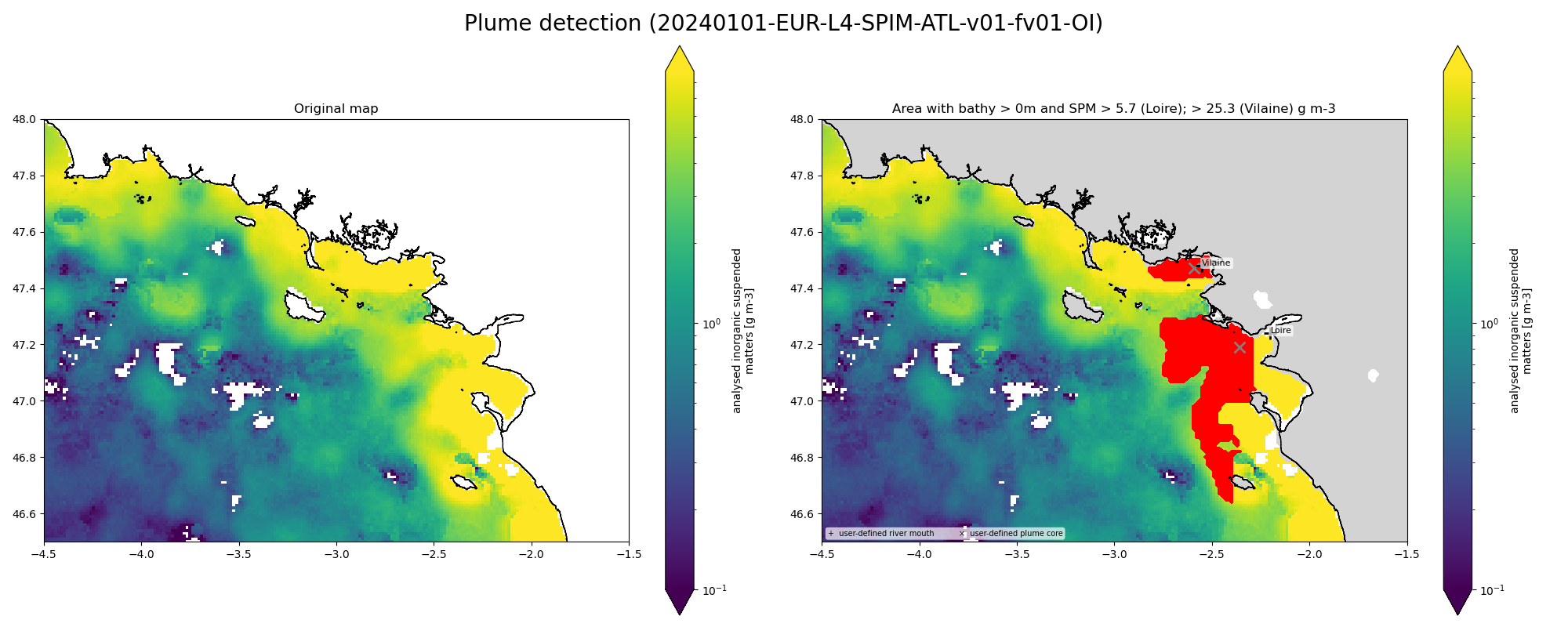
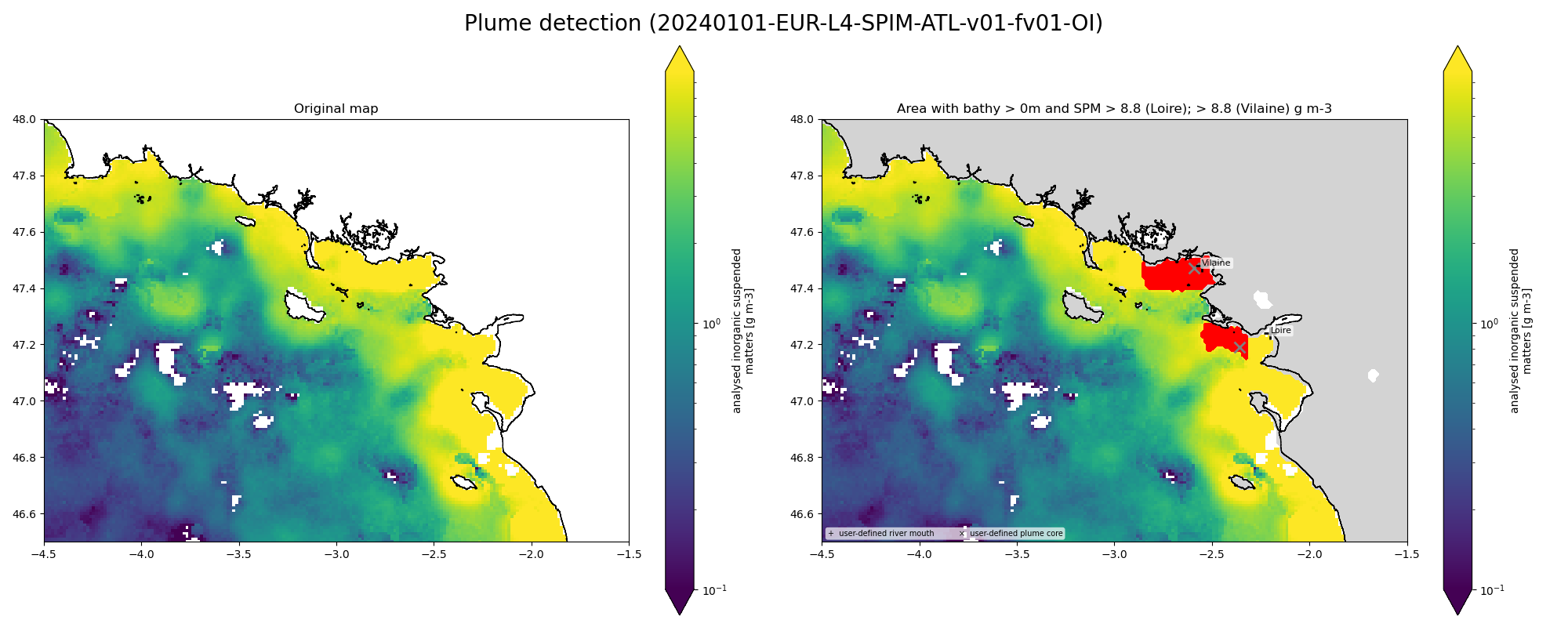
Each PNG shows two panels: the raw SPM field (left) and the detected plume
mask (right), colour-coded per river using a small palette of red shades with
a legend at the bottom of the figure identifying which shade belongs to which
river. Black + markers mark the river-mouth starting points; grey ×
markers show the plume core coordinates.
Note
The screenshots throughout this vignette were captured before the v0.5.0 per-river colour rendering was added, so the plume mask in each image below still appears as a single flat red region rather than one shade per river. The schema and colouring described above reflect the current behaviour.
4. Zone outputs — winter vs summer, dynamic vs p95#
Note
All detections below are based on a single day of satellite data. Results from
a single day can be sensitive to transient conditions (cloud cover, storm
resuspension, river-discharge spikes). More stable, representative plume
statistics are obtained by running panache over a longer time series and
summarising the Results.csv output.
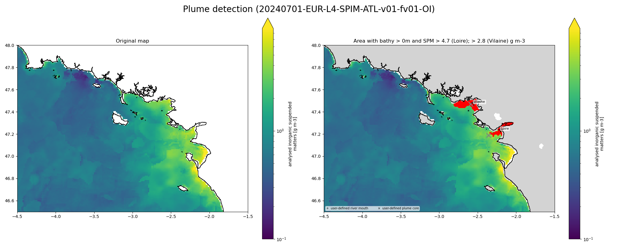
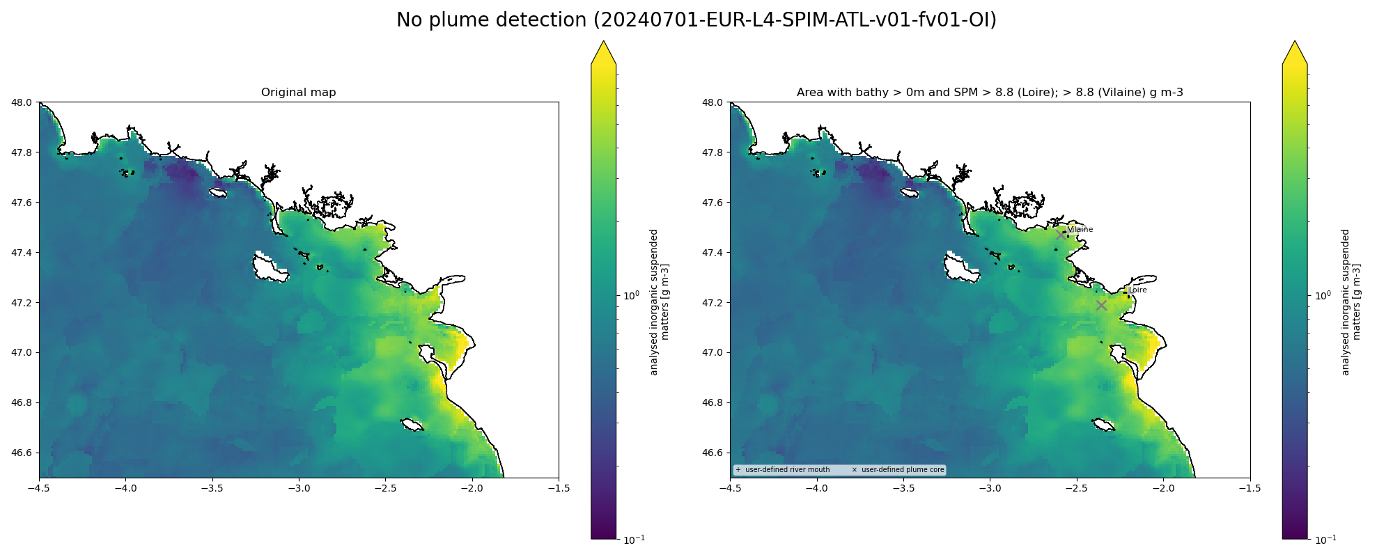
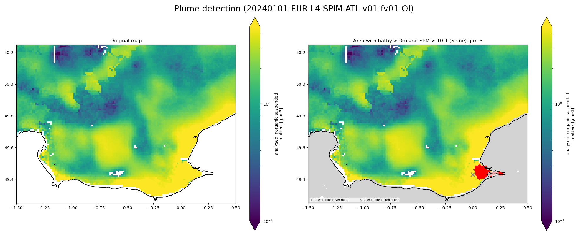
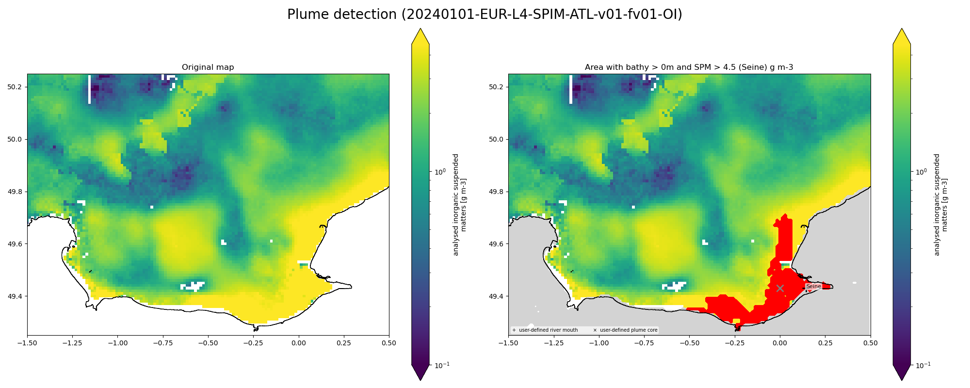
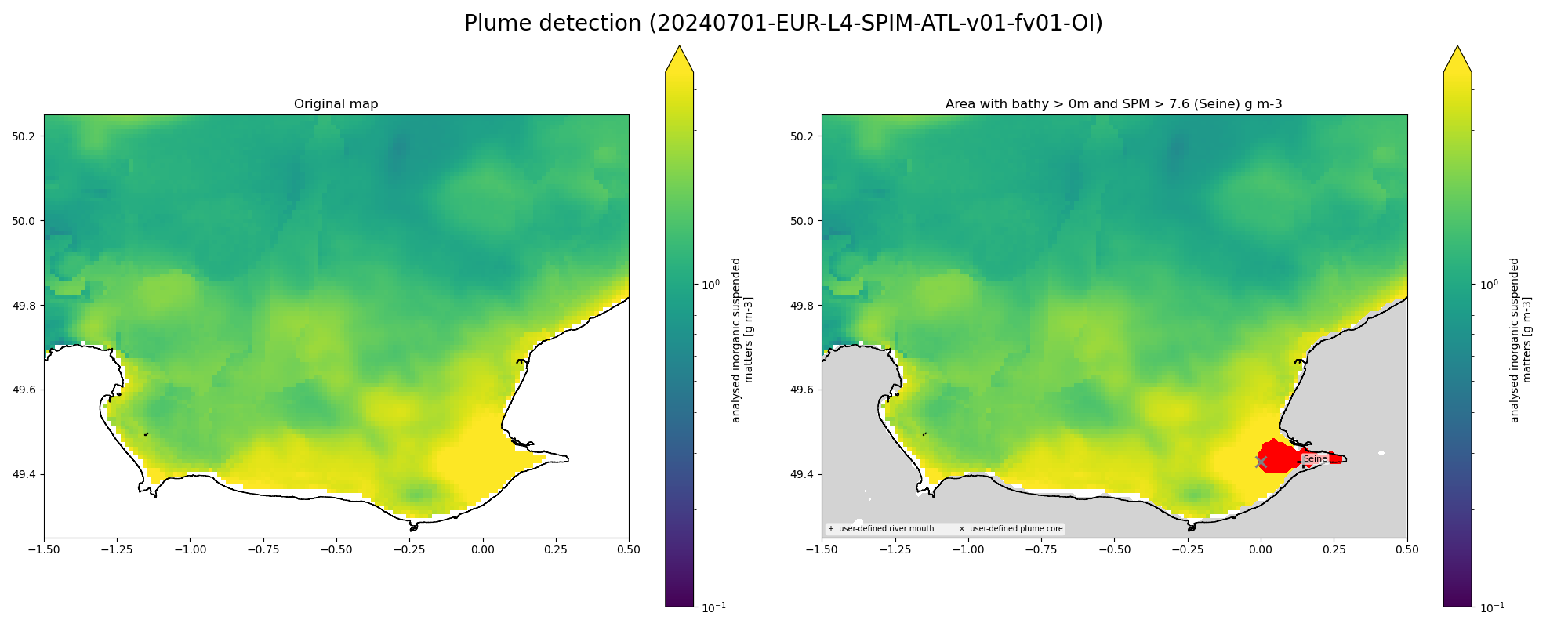
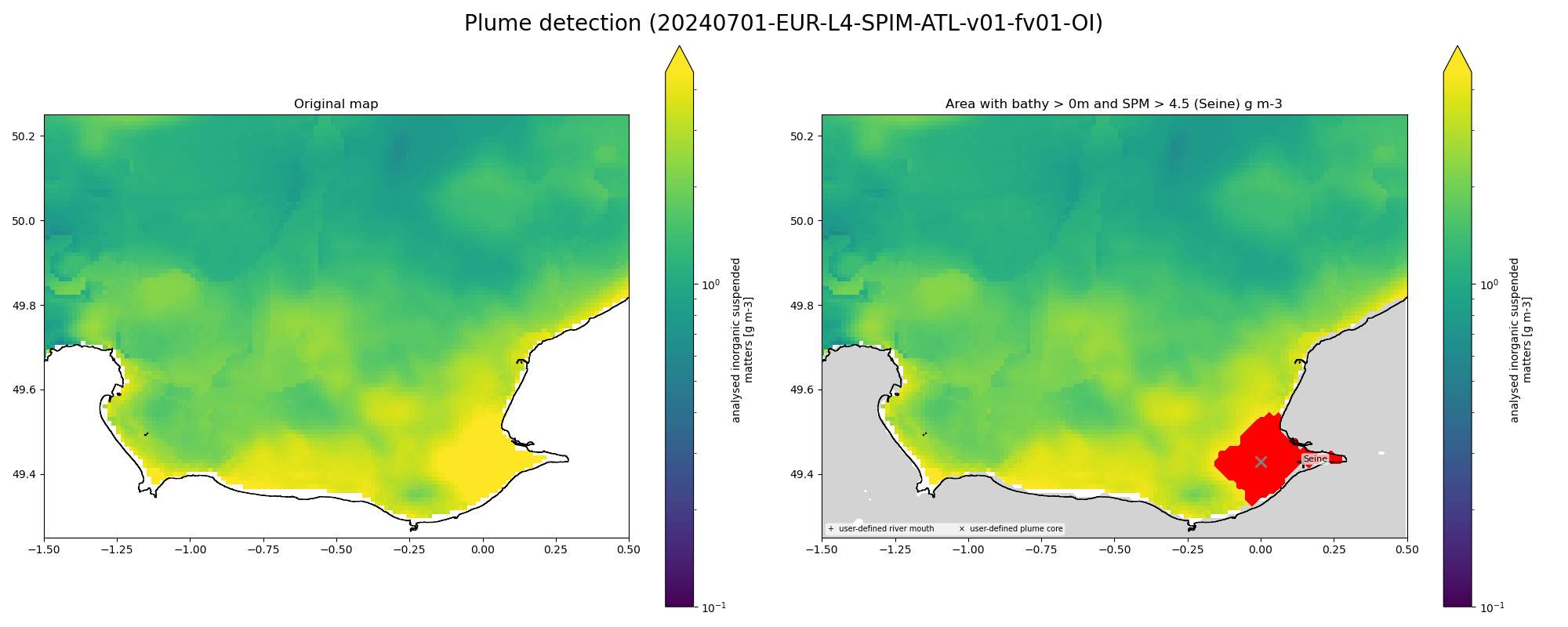
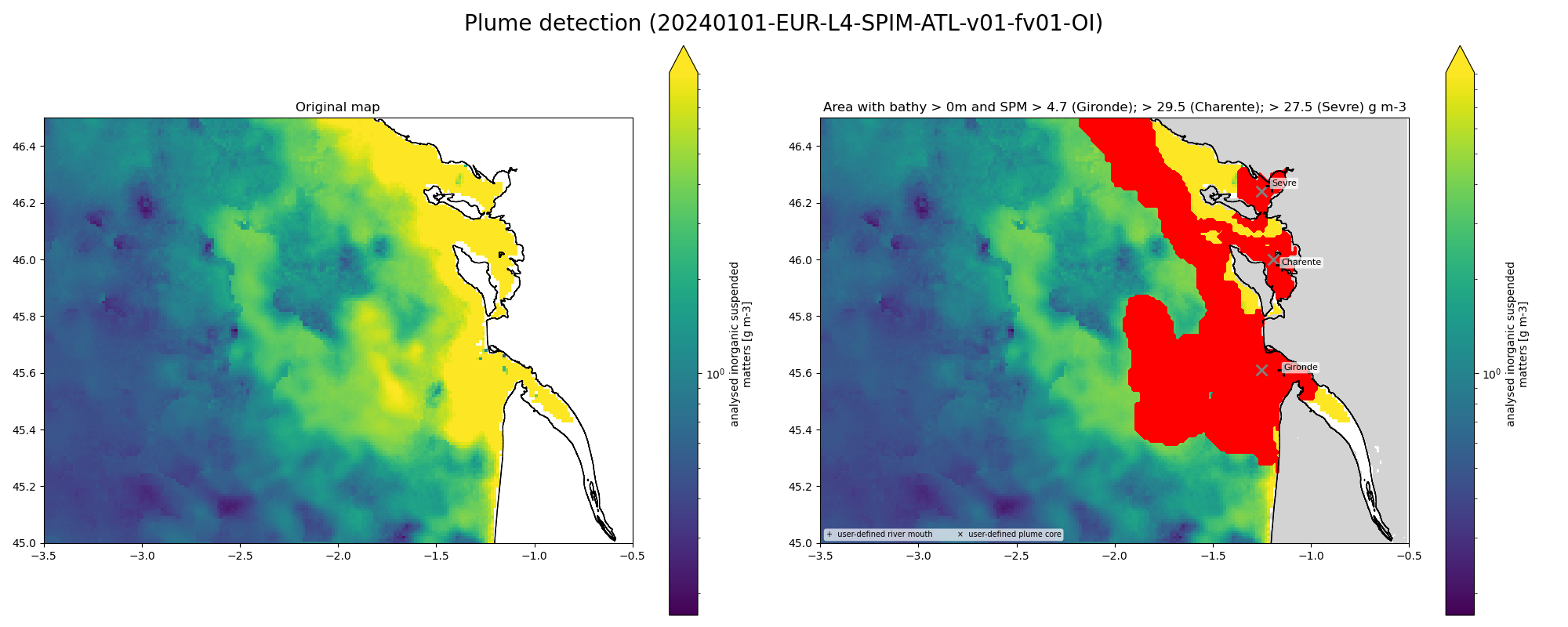
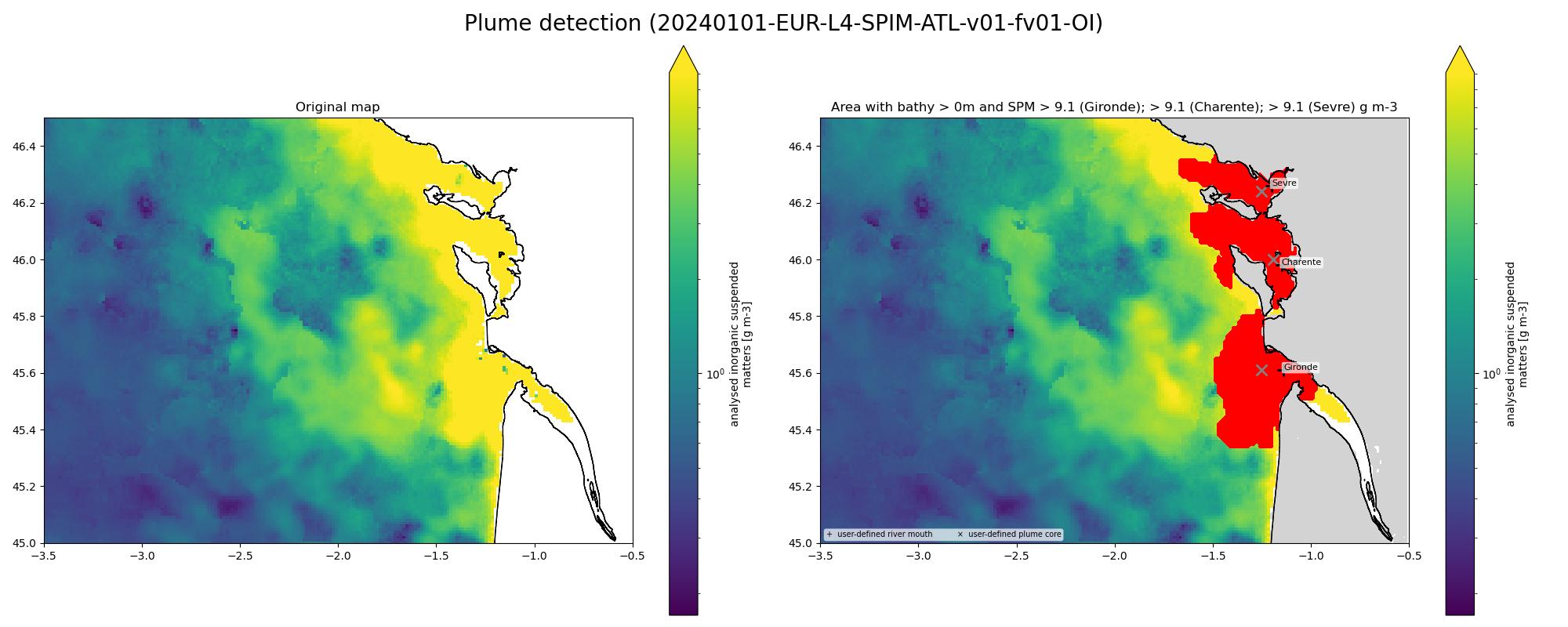
The four panels for each zone share the same colour scale. The plume mask threshold (shown in the right-panel title) differs between the dynamic and p95 runs, illustrating how threshold choice affects the detected plume area.
Bay of Seine#
The Seine estuary opens onto the eastern English Channel. Winter brings high river discharge and elevated SPM; summer discharge is lower and the plume footprint contracts. The bathymetric mask excludes very-shallow tidal flats near the Canal de Caen.
1 January 2024 — Winter
1 July 2024 — Summer
Bay of Biscay#
Three river mouths are tracked simultaneously: the Gironde, the Charente, and the Sèvre Niortaise. The large Gironde plume typically dominates the northern shelf; winter cloud cover (shown as white patches in the left panel) can partially obscure the signal.
1 January 2024 — Winter
1 July 2024 — Summer
Gulf of Lion#
The Grand Rhône and Petit Rhône are tracked as two separate river mouths. The Mediterranean receives less riverine input in summer, and the plume footprint is typically smaller and more confined to the immediate coastal zone. The dynamic threshold adapts per plume per scene; the p95 threshold is a single value computed from the full bounding box.
1 January 2024 — Winter
1 July 2024 — Summer
Southern Brittany#
The Loire and Vilaine are the two tracked mouths. The Loire is one of France’s largest rivers by discharge; the p95 threshold computed from summer data can sometimes exceed ambient SPM concentrations in low-flow conditions, resulting in no plume detected — a physically meaningful result rather than an error.
1 January 2024 — Winter
1 July 2024 — Summer